Quant. Gen. I: From one locus to many

\[ \def\mathbi#1{\textbf{\em #1}} \def\mbf#1{\mathbf{#1}} \def\mbb#1{\mathbb{#1}} \def\mcal#1{\mathcal{#1}} \newcommand{\bo}[1]{{\bf #1}} \newcommand{\tr}{{\mbox{\tiny \sf T}}} \newcommand{\bm}[1]{\mbox{\boldmath $#1$}} \newcommand{\norm}[1]{\left\lVert#1\right\rVert} \DeclareMathOperator{\E}{\mathbb{E}} \DeclareMathOperator{\Var}{\text{Var}} \DeclareMathOperator{\Cov}{\text{Cov}} \DeclareMathOperator{\Corr}{\text{Corr}} \]

Quantitative traits

For practical reasons most early work in genetics relied heavily on physical markers¹. Classic examples include flower color, eye color (Drosophila), …

¹ physical markers: clear, obvious, easy-to-detect, discrete phenotypic differences between individuals.

Figure 1: Physical markers and discrete polymorphisms (photo credits²).

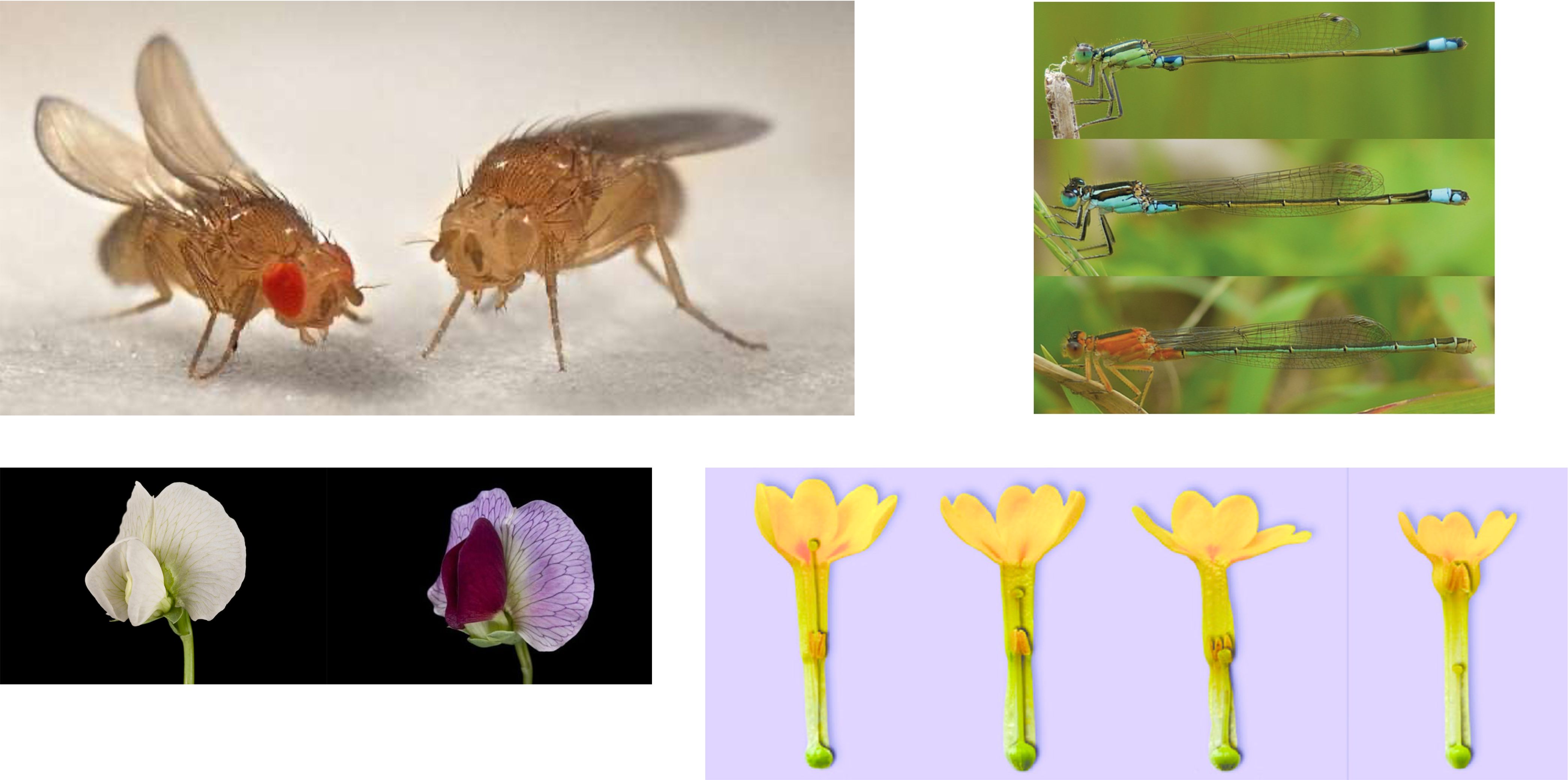
² Clockwise from upper left: Creative Commons Joe Jimbo, Fig.1 from Takahashi et al. 2018, Fig.5 from Brys & Jacquemyn 2015, Science Learning Hub – Pokapū Akoranga Pūtaiao, The University of Waikato Te Whare Wānanga o Waikato

Physical markers made it easy to investigate the segregation ratios of different phenotypes, from which a geneticist could and deduce the genetic underpinnings. BUT these kinds of obvious markers are relatively rare in natural populations. Most phenotypic variation is quantitative. So, how to we go from the basic Laws of Mendelian inheritance at single loci, to the pervasive quantitative variation we see in the nature world?

Figure 2: A famous illustration of quantitative variation in height. Women are dressed in white, men in blue (Photo: Linda Strausbaugh/University of Connecticut, 1996).

To fully appreciate and understand the study of quantitative traits, or quantitative genetics, it is essential to understand a crucial period in the history of evolutionary biology which laid the foundations for theoretical population genetics, and unified Mendelian inheritance and the evolution of quantitative traits.

The battle between the Mendelians and the Biometricians

The story of how the foundations of modern evolutionary biology were laid down begins with attempts to answer this question in the late 1800’s. It also reflects an ongoing conceptual divide between the fields of population and quantitative genetics that unfortunately persists to this day. Today, we will follow the footsteps of the early pioneers of evolutionary genetics as they tried and fought to reconcile how inheritance worked, and how Mendelian inheritance can explain the pervasive quantitative variation in natural populations.

Shortly after the rediscovery of Mendel’s crossing experiments and laws of inheritance in 1900 a major conflict arose between between two factions in evolutionary biology: The Mendelians and the Biometricians.

• 1859 - Origin of Species published. – Sought to explain all variation, from major discrete phenotypic variants to quantitative traits with the same evolutionary mechanism: natural selection. – Didn’t have a working theory of inheritance. + In fact, Darwin and his contemporaries subscribed to so pretty bizarre theories of inheritance! – Highlighted mechanism of inheritance as the major mystery to uncover.

Figure 3: An homunculus, symbol of preformationism (Preformation, drawn by N. Hartsoecker 1695)

• 1900 - Mendel’s work is rediscovered, sparking the controversy between the Mendelians and the Biometricians.

Figure 4: Gregor Mendel (1822 - 1884) (photo credit)

• The real question over which they disagreed was whether evolution proceeded in general by natural selection operating on small variations, as Darwin believed, or by major discontinuous leaps, as both Huxley and Galton believed.

Figure 5: Francis Galton (1822 – 1911) (photo credit)

• During late 1800’s Sir Francis Galton had been struggling to understand inheritance. – Galton remained aloof during the conflict, though he was a central figure because both groups viewed him as their founder. – Believed evolution acted on discontinuous mutations, but also encouraged those working on quantitative variation – in 1893, Galton founded, with W.F.R. Weldon, a Committee for the Royal Society: + “The committee for conducting statistical inquiries into the measurable characteristics of plants and animals”. + He fatefully invited several combustible personalities that fueled the conflict.

The Biometricians

Figure 6: Walter Frank Raphael Weldon (1860 - 1906) (photo credit)

Figure 7: Karl Pearson (1857 – 1936) (photo credit)

• Karl Pearson came from a background in mathematics, but was drawn into the evolution debate by reading Galton’s book Natural Inheritance. Pearson became a friend and colleague of Weldon’s, and followed carefully in Darwin’s footsteps.

“It cannot be too strongly urged that the problem of animal evolution is essentially a statistical problem…(!)”

• Together, Pearson and Wheldon primarily focused on quantitative traits (e.g., height). – Together, they developed the field of “Biometry” – the foundations of modern statistics!
  • A variety of common statistical methods were developed during this time, including correlation analysis (think Pearson’s correlation coefficient) and linear regression.
• Viewed Mendelian inheritance as inextricably linked with discontinuous variation/mutations, and sought an alternative theory of inheritance that made more sense for the continuous characters they were primarily interested in.
  • This led them to develop some strange theories of inheritance, e.g., “homotyposis”.
• Both Pearson & Weldon were involved in The Committee formed by Galton, but consistently butted heads with another member… the acrimony escalated over the years to eventually become lifelong enmity between them.

The Mendelians & William Bateson

• William Bateson was arguably one of the most influential personalities in evolutionary biology.
• He was a bit of a malcontent even in childhood; always extremely sensitive to criticism, with a habit of responding quickly and sharply to any perceived critics.
• He was also particularly poor at mathematics… a shortcoming that he was particularly sensitive, and which had a large impact on his interactions with Wheldon and Pearson.
• Bateson became interested in biology, and studied lakes in the Russian steppes that varied in salinity. He found no general rule for the effect of salinity on animal characteristics, and thought animals could revert to earlier forms if moved between lakes. – This work planted seed of doubt in his mind that Darwin’s idea of selection acting on small variations could actually work.

Figure 8: William Bateson (1861 – 1926) (photo credit)

• Over time, he became convinced of the importance of discontinuous characters as the only way for evolution to proceed at a reasonable pace

  • When Mendel’s crossing studies were rediscovered in 1900 by Hugo de Vries… Bateson immediately latched onto the idea of Mendelian inheritance and the evolution of discrete characters as the only reasonable explanation for how evolution works. – But he made a critical logical error in assuming that Mendelian inheritance requires Major Mutations to produce discontinuous characters.

• His difference of opinion, which emerged in discussions with his biometrical co-committee members escalated.

  • Throughout his career, he vociferously attacked just about everything Weldon published.

• Despite his open contempt for W.F.R. Wheldon, Bateson tried to win Pearson over to Mendelism (mostly for his math skills), but never succeeded.

• Inevitably responded to any rebuttal or critique with more antagonism (even when Weldon or Pearson were only defending themselves against his critiques!)

• But the confusion went both ways, and the conflict was compounded by Weldon’s misinterpretation of Mendel’s work.

Johannsen & Pure Line Theory

• The danish botanist Wilhelm Johannsen enters the fray in the early 1900’s.
• Johannsen studied natural selection using self-compatible bean varieties.
• He created “pure lines” through multiple generations of selfing.
• Curiously, he still saw phenotypic variation in his pure lines, though less than original varieties.
• In 1910, Johannsen performed a series of selection experiments using pure lines and hybrids… the experiments showed: – That selection on traits only went so far before hitting a limit. – That a lot of the small variation in pure lines was not heritable. – That in mixed populations, selection isolated the most phenotypically ‘extreme’ pure line… + Concluded that selection can’t push populations beyond the variation already present³.
• Concluded that his results placed great significance on “discontinuous variation”, which appeared to strongly support the Mendelian’s (i.e., Bateson’s) position.

³ Short Exercise: write out the heterozygote cross table for 3 loci.

Unfortunately, Johannsen, Bateson, and other Mendelians missed a key detail when interpreting the results from some of these experiments. Specifically, Johannsen’s experiments with self-fertilizing pure lines were an example of what we would call ‘clonal selection’ today. That is, since there was only self-fertilization within lines in his experiments, there was no other genotypic variation available for selection to act on (e.g., due to recombination). Had he performed the experiments with outcrossing lines, he would have almost certainly come to a different conclusion

Herman Nilsson-Ehle

Here, we take a moment to highlight a past professor at Lund University who played an important role in this period of history!

Figure 9: Herman Nilsson-Ehle (1873 – 1949) (photo credit)

• Herman Nilsson-Ehle came from a farming family in Southern Skåne (Skurup, born 1873).
• He studied Botany & plant breeding at Lund University.
• In 1900 became assistant to the director of the Swedish Agricultural Experimental Station at Svalöv (now Lantmannen research station).
• Immediately saw the importance of Mendel’s work when it was rediscovered.
  • Led him to study the distribution of phenotypes in Wheat & Oats, focusing specifically at kernel color.

Figure 10: A schematic of the 2-factor segregation patterns in Nilsson-Ehle’s experiments.

• Nilsson-Ehle was eventually able to deduced up to three-factor inheritance patterns for oat kernel color traits.
  • His findings represented a critical turning point in the debate.

Nilsson-Ehle’s crucial observations/conclusions were:

1. He made the critical observation that by the time a trait is influenced by 3 mendelian factors (i.e., three genes), the distribution of segregating phenotypes is nearly continuous and indistinguishable from a Normal Distribution, which was central to the statistical methods developed by the Biometricians.
2. He noted that many of what the Mendelians called “mutations” are only new groupings of genetic variants already present in the population which have been shuffled by recombination.
   • He noted that with a 10 factor system, one could have nearly \(60,000\) possible combinations.
3. He proposed that the primary purpose of sexual reproduction must be to increase the possibility of genetic recombinations

A bit of a disclaimer concerning Herman Nilsson-Ehle

H. Nilsson-Ehle founded the Genetics department at Lund University, and is a major reason for the tradition of strong genetics research at Lund University. However, he is also a source of shame for the Department. Nilsson-Ehle became quite heavily involved in the Eugenics movement during the years prior to World War II, and later expressed very pro-Nazi political leanings that ultimately led to him being quietly dismissed from the University.

As with several of the historical figures involved in the development of the field of genetics, we highlight their scientific contributions and the role they played in the history of the field without voicing any support for their (misguided) political opinions.

Ronald Aylmer Fisher

Figure 11: Ronald Aylmar Fisher (1890 – 1962) (Image from Adelaide Digital Library).

R.A. Fisher ultimately ended what by the 1910’s was a fading battle between the Mendelians and the Biometricians by providing a mathematical unification of population and quantitative genetics. Ironically, R.A. Fisher was himself a divisive figure, and was involved in several other academic conflicts and rivalries (most famously with Sewall Wright).

• R.A. Fisher was a student in the early 1900’s, and exhibited a special genius for mathematics.

• He became interested in Evolution after reading Karl Pearson’s series “Mathematical contributions to the theory of evolution.

• By 1916, he published a paper intent on interpreting well-established results of biometry using Mendelian inheritance.

• In 1922, developed a unifying theory examining the evolutionary consequences of Mendelian heredity, with the central assumption that quantitative traits are governed by many loci, each with very small effects on the phenotype.

  – Many of the ideas he later pursued were contained in this paper.

We will not re-derive R.A. Fisher’s model in full… but we will step through the logic as a foundation for understanding quantitative genetics.

1 locus, 2 loci, 3 loci, more…

Let’s start by considering a single-locus, \(\mbf{A}\), with co-dominant alleles that contribute additively to a quantitative trait of interest (e.g., height, or bristle number). Let’s denote the two alternative alleles as \(A_+\) and \(A_-\), and assume that \(A_+\) causes a small increase in the trait, while \(A_-\) causes a small decrease in the trait value. If we examine a heterozygote cross:

Figure 12: Heterozygote cross for a 1-locus additive model.

we end up with the standard \(3\) phenotypic classes and a segregation ratio of \(1:2:1\).

Now let’s add a 2nd locus, \(\mbf{B}\), also with co-dominant alleles with additive allelic effects on the trait (\(B_+\) and \(B_-\)), and look at the results of a heterozygote cross:

Figure 13: Heterozygote cross for a 2-locus additive model.

Now we have \(5\) size classes, and a segregation ratio of \(1:4:6:4:1\).

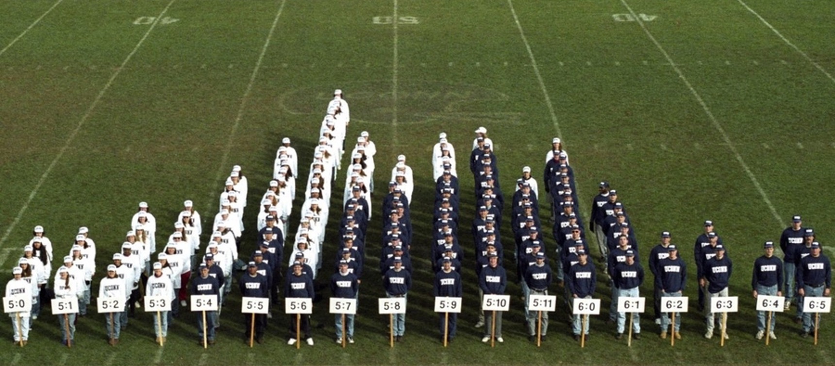
By the time we involve \(3\) loci⁴, we have \(7\) size classes, and a segregation ratio of \(1:6:15:20:15:6:1\). By now, the distribution is starting to look a bit like a bell curve, but with clearly distinguishable phenotypic classes. In the animation (Figure 14) below, we are seeing many possible distributions of phenotypes resulting from a heterozygote cross with \(3\) additive loci contributing to the trait.

⁴ Short Exercise: write out the heterozygote cross table for 3 loci.

Figure 14: Animation showing many possible phenotype distributions among offspring of a heterozygote cross with 3 additive loci influencing the phenotype

Hopefully you can see by now, as Herman Nilsson-Ehle did, that with even relatively few loci contributing to a quantitative trait, the distribution of phenotypes starts resembling the kind of quantitative variation the Biometricians were focused on.

So far, we have assumed that phenotypes are entirely determined by an individual’s genotype. Let’s relax that assumption now, and assume that the environment can introduce as small amount of variation around the genetically determined phenotype:

Figure 15: And now, phenotype distributions resulting from the same 3 additive loci, but with a small amount of additional variation due to the environment.

As you can see, even a little bit of additional variation in the phenotypes due to environmental effects abolishes the clear distinctions between the phenotypic classes. In the end, we have a continuous distribution that is nearly indistinguishable from a normal distribution, or ‘bell curve’… which is exactly what the biometricians would have called a ‘quantitative character’.

So what is quantitative variation?

1. Several loci, \(\mbf{A}\), \(\mbf{B}\), \(\mbf{C}\), … \(\mbf{n}\)
2. Each with alternative alleles: \(A^+\), \(A^−\), \(B^+\), \(B^−\), \(C^+\), \(C^−\), … that contribute additively to a given trait… one increasing the trait’s value, the other decreasing it.
3. Each locus has limited effect, and contribute additively to the overall trait value.
4. Environmental variation “blurs” the edges of the realized phenotypes for the genotype classes.
5. 1918,1922: R.A. Fisher formally shows that as the number of loci becomes large, and each has a small effect on the phenotype, all previous results from the Biometricians can be explained by this model, which relies solely on Mendelian inheritance!
6. By ∼1930 The synthesis of Mendelian and Quantitative trait evolution is formally resolved within the overarching framework of Theoretical Population Genetics.

Important consequences:

1. Based on a quantitative trait, you cannot know what genotype corresponding to a given phenotypic value.
2. Therefore, we must shift our focus to an analysis of phenotypes rather than genotypes.
   • Phenotypes must be measured and analyzed using statistical methods rather than genetic.
3. Interestingly, even though the Biometricians were ultimately wrong about how inheritance worked, the statistical methods they developed were – and continue to be – essential tools for analyzing genetic data!