Pop. Gen. I: Genetic Variation
\[ \usepackage{amsmath} \usepackage{amssymb} \def\mathbi#1{\textbf{\em #1}} \def\mbf#1{\mathbf{#1}} \def\mbb#1{\mathbb{#1}} \def\mcal#1{\mathcal{#1}} \newcommand{\bo}[1]{{\bf #1}} \newcommand{\tr}{{\mbox{\tiny \sf T}}} \newcommand{\bm}[1]{\mbox{\boldmath $#1$}} \newcommand{\norm}[1]{\left\lVert#1\right\rVert} \DeclareMathOperator{\E}{\mathbb{E}} \]
A little bit of history
Although it seems trivial today, the problem of explaining how inheritance worked was THE major obstacle facing Darwin as he was developing his theory of evolution by natural selection. Darwin and other thinkers of the time could all see as plainly as we can that offspring resemble their parents more than they do some other randomly chosen individual… but WHY? HOW?
They came up with some pretty interesting theories, including:
- Pangenesis: Every cell in an organism emitted small particles, which were units of heredity, that Darwin called gemmules. The gemmules could either circulate and disperse in the body system, or they could aggregate in the sexual cells located in reproductive organs. As hereditary units, the gemmules transmitted from parents to offspring, where they developed into cells that resembled the parents’ cells. It was not sexual cells alone that generated a new organism, but rather all cells in the body as a whole.
- Preformation: Embryos spring into existence fully formed, but microscopic in size.
- Blending Inheritance: The unsatisfactory theory of choice for Darwin and several of his contemporaries. In fact, Darwin’s version of Blending Inheritance was a variation of pangenisis, where he assumed the gemmules from a mother and father combined to produce an offspring of intermediate phenotype.
- Variation among siblings could then be explained by random variation in the composition of gemmules inherited by each sibling

There is an inherent problem with the idea of blending inheritance. Do you see it?
Take a minute to pause and ponder. Consider the extreme case where, for example, children grow up to be intermediate in height relative to their two parents. What happens to the variance in height over several generations?
Hopefully, you can see that blending inheritance would lead to a rapid regression to the mean and loss of 1/2 of the variance in height in each generation. Our hypothetical population would very quickly evolve so that all individuals were exactly the same height, which would be exactly equal to the mean height in the first generation! Clearly, this did not conform the the tremendous variation Darwin observed in natural populations. Nevertheless, he had not better alternative theory to offer.
Darwin’s (reluctantly) favoured theory – blending inheritance – offers some insight into his early vision of how evolution by natural selection worked. Blending inheritance would rapidly reduce variation, which needed to be constantly regenerated somehow. There were two main mechanisms that could generate such variation. One was spontaneous mutation; the other was alteration of phenotypes by interactions between organisms and their environment, which Darwin viewed as infinitely variable due to geologic processes. Here we can already see the seeds of his theory of natural selection taking shape. Nevertheless, he was confounded by the re-emergence of ancestral forms in pedigrees (i.e., offspring that more closely resembled a great-great-grandparent than their parents)… if blending inheritance was destroying variation, how were these ancestral forms being reconstituted in later generations?
Darwin was also plagued by an inability to fully reconcile ’sports’ and ’minor variants’, known today as discrete phenotypes/large-effect mutations and quantitative variation, respectively. The rediscovery of Gregor Mendel’s breeding experiments in 1900 provided key answers. Mendel had deduced the existence of “heritable factors”, from the distribution of offspring phenotypes from controlled parental crosses. These heritable factors which later came to be known as chromosomes.

But how could these heritable Mendelian factors explain ALL the observable phenotypic variation in real populations, most of which is quantitative rather than discrete? Understanding the generation and maintenance of genetic variation is “the great obsession” of population geneticists (Gillespie 2004).
Over the next 30 years the field of population genetics ‘coalesced’, with the main goal of explaining how genetic variation is created, maintained, and shaped by evolutionary processes. A pantheon of important characters played critical roles in the development of the field. Titanic battles were fought, won, lost, forgotten, & remembered. We will meet and highlight a few of these characters over the course of these lectures.
Population genetics was built upon a rich body theory long before the technology to directly study DNA sequences was invented!
A major recent shift: With the advent of modern whole genome sequencing technology, we are now drowning in DNA sequence data. Finding new ways to apply (or extend) classical population genetics theory to analyze modern data is the major current challenge in the field!!!
Everything from modern statistics to bioinformatics is built on the foundations of theoretical population genetics. YOU NEED TO KNOW THIS STUFF! EMBRACE THE MATH!!
Genetic Variation
Some basics
Definitions
- Gamete = reproductive cells (egg, sperm)
- Gametes are Haploid (carry one copy of genome).
- \(n\) is often used as the symbol for the number of chromosomes in a gamete (e.g., \(n = 23\) in humans)
- Homologs = Paired chromosomes in Diploid cells.
- One originating from the maternal gamete, one from the paternal.
- Chromosome = One, linear DNA molecule and associated proteins.
- Locus = A specific position of interest on a chromosome.
- Allele = A unique variant of the same locus.
- Different alleles thus represent different DNA sequences for the specific region in question.
Consider a specific position (may be a small region), locus \(\mbb{A}\), and assume that among all chromosomes of that type within the species, there exist two alternative alleles, \(A_1\) and \(A_2\). A single individual must then have one of the following three genotypes at locus \(\mbb{A}\): \(A_1 A_1\), \(A_2 A_2\), or \(A_1 A_2\). In the first two cases the individual is said to be homozygous and in the last case heterozygous.
Several cycles of mitosis + differentiation without true genetic alteration of cells (i.e., mutation) produces a developed multicellular organism with differentiated organs (e.g. brain, liver etc). All cells contain the same genetic information (ignoring somatic mutations)! Mitosis continue as long as the individual lives.
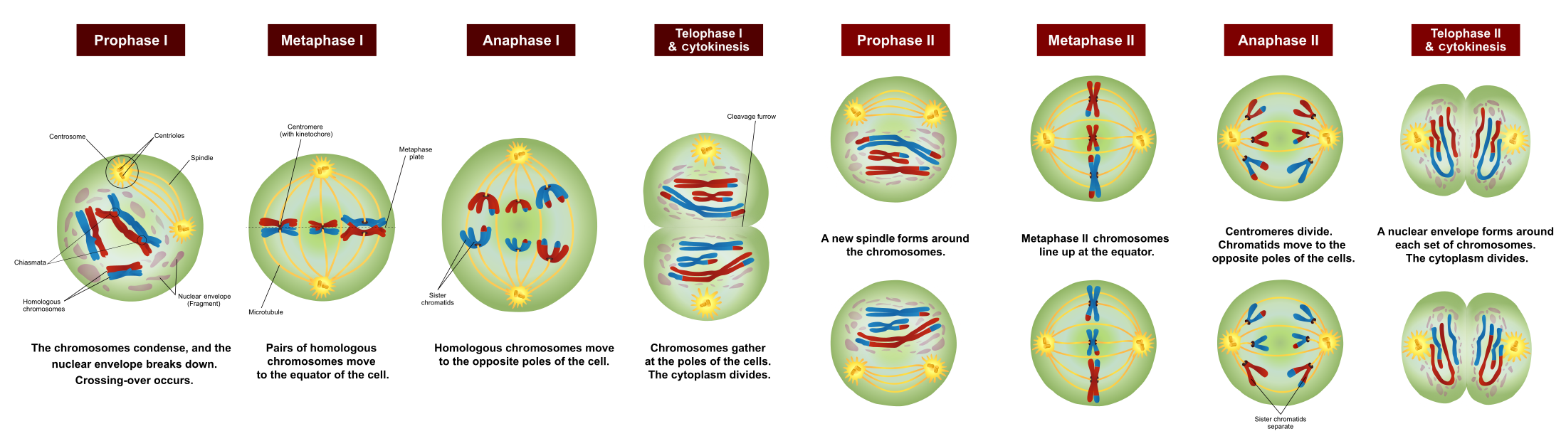
In reproductive organs, (ovaries/testes in animals, ovaries/anthers in flowering plants), a specific type of cell division occurs: Meiosis. Meiosis involves a 2nd cellular division that reduces the ploidy of the daughter cells from diploid (\(2n\)) to haploid (\(n\)). These haploid daughter cells are Gametes.
- If an individual is homozygous all of their gametes will carry the allele they are homozygous for (of course!).
- If an individual is heterozygous (\(A_1 A_2\)), half of the gametes will carry \(A_1\) and half will carry \(A_2\).
- This is known as Mendel’s first law. Exceptions occur, but we will ignore them for the most part in this course.
From Genotype to Phenotype
A gene is a stretch of DNA with a function. The phenotype of an individual is, put simply, its detectable properties in the widest sense of the word. The phenotype of an individual is a function of both its genotype at relevant genes and the environment1. Lets consider the simplest case: when the phenotype is determined entirely by an individual’s genotype genotype at a particular gene with a single locus. Let:
1 We will mostly focus on the genetic component of of an individual’s phenotype, and ignore effects of the environment (until our Quantitative Genetics Lectures).
\[ \begin{aligned} \text{Phenotype of } A_1A_1 &\rightarrow Ph_1 \\ \text{Phenotype of } A_1A_2 &\rightarrow Ph_{12} \\ \text{Phenotype of } A_2A_2 &\rightarrow Ph_2 \end{aligned} \]
- If \(Ph_1 < Ph_{12} < Ph_2\), then the alleles \(A_1\) and \(A_2\) are said to have an intermediate mode of inheritance (sometimes called semi-dominance).
- If \(Ph_1 = Ph_{12} \neq Ph_2\), the \(A_1\) allele is said to have a dominant mode of inheritance, and \(A_2\) allele is said to have a recessive mode of inheritance.
- \(Ph_1 \neq Ph_{12} = Ph_2\) would represent the opposite dominance relationship.
With intermediate modes of inheritance, all genotypes produce a unique phenotype. This is not the case when one allele is recessive:

Genotype & Allele Frequency Calculations
Definitions
- Allelic richness = the number of alleles currently segregating at a given locus.
- Genetic Diversity Index = Expected heterozygosity = the probability that 2 randomly drawn gene copies are of different alleles.
Consider a single diploid locus, \(\mbb{A}\) in a diploid population with two alternative alleles, \(A_1\) and \(A_2\). To calculate the frequency of each allele, we would use the following formulae:
\[ \begin{aligned} fr(A_1) = \frac{2 \times n_{A_1 A_1} + n_{A_1 A_2}}{2 N} \\ fr(A_2) = \frac{2 \times n_{A_2 A_2} + n_{A_1 A_2}}{2 N} \end{aligned} \]
where \(n_{ij}\) (and \(i \in \{A_1,A_2\}\)) denotes the number of individuals of genotype \(ij\), and \(N\) is the total number of individuals sampled. Note that \(fr(A_2) = 1 - fr(A_1)\), so that the frequencies always sum to one.
| \(A_1A_1\) | \(A_1A_2\) | \(A_2A_2\) | \(\sum\) | |
|---|---|---|---|---|
| \(n\) | \(158\) | \(44\) | \(67\) | \(269\) |
| \(\text{Genotype Freq.}\) | \(\frac{158}{269} = 0.587\) | \(\frac{44}{269} = 0.164\) | \(\frac{67}{269} = 0.249\) | \(1.0\) |
What about the frequency of the \(A_1\) and \(A_2\) alleles? Applying the equations for allele frequencies above to the above example, we have2:
2 Note that we have labeled the alternative allele frequencies \(p\) and \(q\), such that \(q = 1 - p\). We will use this convention throughout the course.
\[ \begin{aligned} fr(A_1) = p &= \frac{(2 \times 158) + 44}{2 \times 269} = 0.669 \\ fr(A_2) = q &= \frac{(2 \times 67) + 44}{2 \times 269} = 0.331 \end{aligned} \]
So, how do we quantify genetic variation at this \(\mbb{A}\) locus? There are several ways to do this. For example, one could simply count the number of segregating alleles at a locus, the Allelic richness. However, a far more common and natural way to quantify genetic variation is to use the Genetic diversity index, or Expected Heterozygosity (\(H\)). \(H\) quantifies the probability that 2 randomly drawn gene copies are different alleles3.
3 Consider including the binomial variance here? \(H\) is the standard for quantifying genetic diversity, and is a natural choice: if we consider the allelic state at a given locus to be a random binomial variate, \(H\) is literally the binomial variance of allelic states. Note: more natural derivations of \(H\) and \(\pi\) come in our lecture on finite populations.
\[ \begin{aligned} H &= \sum_{i=0}^{k} 2 p_i(1 - p_i) \\ &= 1 - \sum_{i=0}^{k} p_i^2 \end{aligned} \]
where \(p_i\) is the frequency of the \(i^{th}\) allele, and the summation is over the number of segregating alleles at the given locus (\(k\)).
For DNA sequence data, where we are dealing with many segregating sites, we quantify heterozygosity using \(\pi\) (\(\pi \approx 0.001\) in humans).
\[ \begin{aligned} \pi &= \E \left[ \sum_{i=0}^{\infty} 2 p_i(1 - p_i) \right] \\ &= \E \left[ \sum_{i=0}^{\infty} 1 - p_i^2 \right] \end{aligned} \]
where here \(p_i\) denotes the frequency of the major allele (with highest frequency) at the \(i^{th}\) site in the genome.
So, what is the genetic diversity at the \(\mbb{A}\) locus? \(H_{\mbb{A}} = 2p(1-p) = 2 p q = 0.443\).
Consider a 2nd locus, \(\mbb{B}\) with \(4\) alleles:
\(fr(B_1) = 0.9\), \(fr(B_2) = 0.05\), \(fr(B_3) = 0.025\), \(fr(B_4) = 0.025\).
Which locus has more genetic variation, \(\mbb{A}\) or \(\mbb{B}\)?
- Using allelic richness, \(\mbb{B}\) has more (\(4\) vs. \(2\) alleles)
- Using expected heterozygosity:
\[ \begin{aligned} H_{\mbb{A}} &= 2p(1-p) = 0.443 \\ H_{\mbb{B}} &= \sum_i^k 1 - p_i^2 = 1 - 0.9^2 - 0.05^2 - 0.025^2 - 0.025^2 = 0.186\\ \end{aligned} \]
The \(\mbb{A}\) locus has fewer alleles, but is more genetically diverse.
Hardy-Weinberg Proportions
A fundamental concept in population genetics is the expected frequency of different genotypes, given a particular allele frequency, in the absence of any other evolutionary forces. That is, if allele \(A_1\) is at frequency \(p\), what are the expected frequencies of the three genotypes \(A_1A_1\), \(A_1A_2\), and \(A_2A_2\) in the absence of mutation, selection, drift, or migration? A simple approach to calculating these expected frequencies is to make the simplifying assumption that mating occurs at random. Or more specifically, that each zygote is formed by the union of two haploid gametes drawn at random based on their frequencies in the parental generation. In this idealized case, the expected genotypic frequencies among offspring can be treated as binomial variables, where the probability of forming each genotype is the product of the frequencies of the alleles composing the genotype. These Hardy-Weinberg frequencies are summarized in the table below:
| \(A_1A_1\) | \(A_1A_2\) | \(A_2A_2\) | \(\sum\) | |
|---|---|---|---|---|
| \(n\) | \(158\) | \(44\) | \(67\) | \(269\) |
| \(\text{Genotype Freq.}\) | \(\frac{158}{269} = 0.587\) | \(\frac{44}{269} = 0.164\) | \(\frac{67}{269} = 0.249\) | \(1.0\) |
| \(\text{Expected Gen. Freq.}\) | \(p_1^2\) | \(p_1 p_2 + p_2 p_1 = 2p_1 p_2\) | \(p_2^2\) | \((p_1 + p_2)^2 = 1.0\) |
| \((p_1 = p,\, p_2 = q)\) | \(p^2\) | \(2pq\) | \(q^2\) | \((p + q)^2 = 1.0\) |
Note that the expected frequencies generalize to more than two alleles at a given locus.
- If we have alleles \(A_1, A_2, A_3,\ldots,A_n\), with frequencies \(p_1, p_2, p_3,\ldots, p_n\), then:
- Expected frequency of genotype \(A_iA_j\) is \(2 p_i p_j\)
- Expected frequency of genotype \(A_iA_i\) is \(p_i^2\)
Phenylketonuria is a recessive congenital metabolic disease resulting in buildup of the amino acid phenylalynine. Caused by mutations in PAH gene resulting in reduced production of the enzyme phenylalynine hydroxylase. The incidence of PKU is approximately \(1/10,000\). What is the allele frequency?
Since PKU is recessive, and the disease phenotype occurs at a rate of \(1/10,000\), we can infer the frequency of the disease allele (let’s call it \(A_2\)) as follows:
\[ f(A_2A_2) = q^2 = \frac{1}{10,000} \]
Therefore,
\[ q = \sqrt{\frac{1}{10,000}} = \frac{1}{100} \]
We can summarize using a similar table as above:
| \(A_1A_1\) | \(A_1A_2\) | \(A_2A_2\) | |
|---|---|---|---|
| HW | \(p^2\) | \(2pq\) | \(q^2\) |
| PKU | \(p^2\) | \(2(1 - \frac{1}{100})\frac{1}{100}\) | \((\frac{1}{100})^2\) |
| \(2(\frac{1}{100} - \frac{1}{100^2})\) | \(\frac{1}{10,000}\) | ||
| \(\approx \frac{2}{100} = \frac{1}{50}\) | \(\frac{1}{10,000}\) |
Insight: Where do we find rare alleles? in heterozygotes!
If locus \(\mbb{A}\) is X-linked, the genotypic probabilities in females follow the same expected proportions as for an autosomal genes (\(p^2, 2pq, q^2\)). But for species with an X-Y sex determination system, males are either \(A_1Y\) or \(A_2Y\), so their genotype frequencies are simply \(p\) and \((1 - p)\). Consider color blindness, which occurs in males at a frequency of \(\approx 7\%\)4
\[ \begin{aligned} p &= 0.07 = 7/100 \\ p^2 &= 0.0049 \approx 1/2000 \end{aligned} \]
4 This example illustrates why color blindness is primarily an issue for males rather than females.
Haplotypes and Linkage Disequilibrium
So far we have focused on a single locus at a time. But obviously, a genome consists of many loci, and we are often interested in describing variation at more than just a single locus at a time. To do this, we need to define haplotypes5
5 Haplotypes: the specific set of alleles residing at multiple loci on the same chromosome.

Consider a chromosome with two loci, \(\mbb{A}\) (with alleles \(A_1, A_2\)) and \(\mbb{B}\) (with alleles \(B_1, B_2\)) residing on it. There are four possible combinations of alleles that may reside on the same chromosome:
| \(\text{Haplotypes}\) | \(\text{Frequencies}\) | \(\text{Freq. if independent (r = 1/2)}\) |
|---|---|---|
| \(A_1B_1\) | \(x_{11} = p_1q_1 + D\) | \(p_1q_1\) |
| \(A_1B_2\) | \(x_{12} = p_1q_2 - D\) | \(p_1q_2\) |
| \(A_2B_1\) | \(x_{21} = p_2q_1 - D\) | \(p_2q_1\) |
| \(A_2B_2\) | \(x_{22} = p_2q_2 + D\) | \(p_2q_2\) |
Note that we are using \(p_i\) to denote allele frequencies at the \(\mbb{A}\) locus and \(q_i\) to denote allele frequencies at the \(\mbb{B}\) locus:
\[ \begin{array} f(A_1) = p_1 & f(B_1) = q_1 \\ f(A_2) = p_2 & f(B_2) = q_2 \end{array} \]
We can now formally define Linkage Disequilibrium as the statistical correlation between allelic states at these two loci6:
6 We will revisit Linkage Disequilibrium in more detail in Lecture V.
\[ D = x_{11} x_{22} - x_{12} x_{21} \]
Note: If the allelic states at the loci are independent (i.e., there is no LD), then:
\[ \begin{aligned} D &= p_1 q_1 \cdot p_2 q_2 - p_1 q_2 \cdot p_2 q_1 \\ &= p_1 q_1 p_2 q_2 - p_1 q_2 p_2 q_1 \\ &= 0 \end{aligned} \]
Recombination breaks down the statistical association between loci by randomly ’swapping’ alleles between homologous chromosomes during meiosis I. This happens all the time, but it only matters when it happens in double heterozygotes.
Work in small groups of 2-4. Draw out an illustration of why only recombination between double heterozygotes will affect LD
We can describe the per-generation decay in LD due to recombination as follows:
\[ \begin{aligned} D^{\prime} &= D(1 - r) \\ D_{t+1} &= D_t(1 - r) \end{aligned} \]
and a general solution for the decay of LD follows: \[ \begin{aligned} D_t &= D_0 (1 - r)^t \\ &\approx D_0 e^{-rt} \\ \end{aligned} \]
- Genetics as a field started off extremely data poor, with major challenges related to understanding how inheritance works. This led to the development of a rich body of theory, with little empirical data with which to test it. Now, the problem is reversed! We are drowning in genomic data, and the major challenge is learning how to adapt existing theory (or develop new theory) to analyze it all!
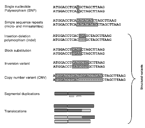
- Different types of genetic variation, and the mapping from genotype to phenotype.
- Genotype and allele frequency calculations for autosomal and sex-linked loci.
- Quantifying genetic diversity - the genetic diversity index, \(H\), allelic richness, etc.
- Independent segregation, random (binomial) gamete sampling, and H-W proportions.
- Linkage disequilibrium, and how recombination breaks it down over time.