Pop. Gen. V: Selection at two loci
\[ \def\mathbi#1{\textbf{\em #1}} \def\mbf#1{\mathbf{#1}} \def\mbb#1{\mathbb{#1}} \def\mcal#1{\mathcal{#1}} \newcommand{\bo}[1]{{\bf #1}} \newcommand{\tr}{{\mbox{\tiny \sf T}}} \newcommand{\bm}[1]{\mbox{\boldmath $#1$}} \newcommand{\norm}[1]{\left\lVert#1\right\rVert} \DeclareMathOperator{\E}{\mathbb{E}} \DeclareMathOperator{\Var}{\text{Var}} \DeclareMathOperator{\Cov}{\text{Cov}} \DeclareMathOperator{\Corr}{\text{Corr}} \]
Linkage Disequilibrium Revisited
So far, we have discussed Linkage Disequilibrium (LD) rather loosely as an association between alleles at different loci. Here, we revisit LD and present a more formal derivation. It is also worth noting at the beginning that “Linkage Disequilibrium” is perhaps a rather unfortunate term, since genetic linkage is only one of many ways to generate LD. A more appropriate term, which is rarely used today is “gametic phase disequilibrium”. Recall from the first lecture how we quantified LD; consider two loci, \(\mbf{A}\) (with alleles \(A\) and \(a\)), and \(\mbf{B}\) (with alleles \(B\) and \(b\)). We showed that we can quantify LD as follows: \[ \begin{aligned} D &= p_{AB} - p_A p_B \\ &= x_1 x_4 - x_2 x_3 \end{aligned} \]
where \[ \text{Haplotype Frequencies} \left\{ \begin{array}{c} x_1:\, AB \\ x_2:\, Ab \\ x_3:\, aB \\ x_4:\, ab \end{array} \right. \]
LD is a covariance!
LD has a formal mathematical definition: it is a Covariance between the allelic states at two different loci. To derive this results, we start by recognizing that when we have two alternative alleles at each of two loci, we can represent the allelic ‘state’ at each locus on a haplotype as two Bernoulli variables. Consider our two loci \(\mbf{A}\) and \(\mbf{B}\) above, but now we will encode the allelic states (\(A\) or \(a\), \(B\) or \(b\)) as Bernoulli variables \(X\) and \(Y\), each of which can take the values of\(0\) or \(1\). Looking our table of haplotype frequencies above, we can write out the following expectations (means) and variances for \(X\) and \(Y\): \[ \begin{aligned} \E[X] &= x_1 + x_2 = p \\ \E[Y] &= x_1 + x_3 = q \\ \Var[X] &= p(1 -)p \\ \Var[Y] &= q(1 -)q \end{aligned} \]
Note that we are using \(p\) for the frequency of the \(A\) allele at the \(\mbf{A}\) locus, and \(q\) for the frequency of the \(B\) allele at the \(\mbf{B}\) locus. This is different from our earlier 1-locus models, where we followed the convention of \(q = (1 - p\)).
Now, from the definition of a covariance (see our formula sheet), we have: \[ \begin{aligned} D = \Cov[X,Y] &= \E[XY] - \E[X]\E[Y] \\ &= x_1 - pq \\ &= x_1 - (x_1 + x_2)(x_1 + x_3) \\ &= x_1(1 - x_1 + x_2 + x_3) - x_2 x_3 \\ &= x_1 x_4 - x_2 x_3 \\ \end{aligned} \]
Which is identical to the formula above, and which we learned in the first lecture!
You will often see the correlation coefficient, \(r^2\), used to quantify LD when analyzing DNA sequence data. The correlation coefficient is just a standardized measure of the covariance: \[ \begin{aligned} \Corr[X,Y] &= \frac{\Cov[X,Y]^2}{\Var[X]\Var[Y]} \\ r^2 &= \frac{D^2}{p(1-p)q(1-q)} \\ \end{aligned} \]
Causes of LD
In this course, we will discuss four main processes that influence the magnitude of LD1. We will spend the most time on demographic history and selection, and only briefly cover some key results for inbreeding & drift.
1 They are:
- Inbreeding (won’t discuss too much)
- Drift
- Demographic history
- Selection
Inbreeding
Recall that under our generalized model of inbreeding, the genotypic frequencies at any given locus are expected to follow: \[ \begin{aligned} F_{AA} &= p^2 + F p q \\ F_{Aa} &= 2 p q (1 - F) \\ F_{AA} &= q^2 + F p q \end{aligned} \]
where \(F\) is Wright’s inbreeding coefficient. The key point (again) is that inbreeding increases homozygosity (without altering allele frequencies). However, we know that it is only recombination events between double heterozygotes that breaks up LD. Hence, by reducing heterozygosity at multiple loci – and therefore the number of double-heterozygotes – we would expect inbreeding to increase LD by reducing the effective recombination rate. In fact, it can be shown2 that (at least for relatively closely linked loci) the effective recombination rate is: \[ r_{\text{eff.}} = r(1 - F) \]
2 We won’t go through a derivation here.
It is important to remember that, by reducing the effective rate of recombination, inbreeding causes genome-wide LD. This means that loci don’t have to be on the same chromosome to be affected!
Genetic Drift
Drift influences LD in two main ways: One we’ve already covered, the other is more subtle but less important.
- Drift will continuously erode LD via loss of heterozygosity: \(D_t = D_0(1 − r)^t\)
- Alleles at different loci can become associated by chance.
- e.g., the frequencies of the \(A\) and \(B\) alleles at loci \(\mbf{A}\) and \(\mbf{B}\) can randomly fluctuate up or down at the same time.
- This causes a weak genome-wide signal of LD.
- BUT no long-term signal of LD because the same random fluctuations will continuously break down LD.
Demographic History
Population demographic history can influence LD in many ways. Some of the most important include:
- Population bottlenecks can result in particular variants at different loci being correlated.
- Rapid population expansions/contractions can cause a buildup of LD relative to its’ rate of decay due to recombination)
- Admixture generates LD if two populations with different haplotype frequencies combine to form one (initially) heterogeneous populations.
We will focus on Admixture by way of an example.
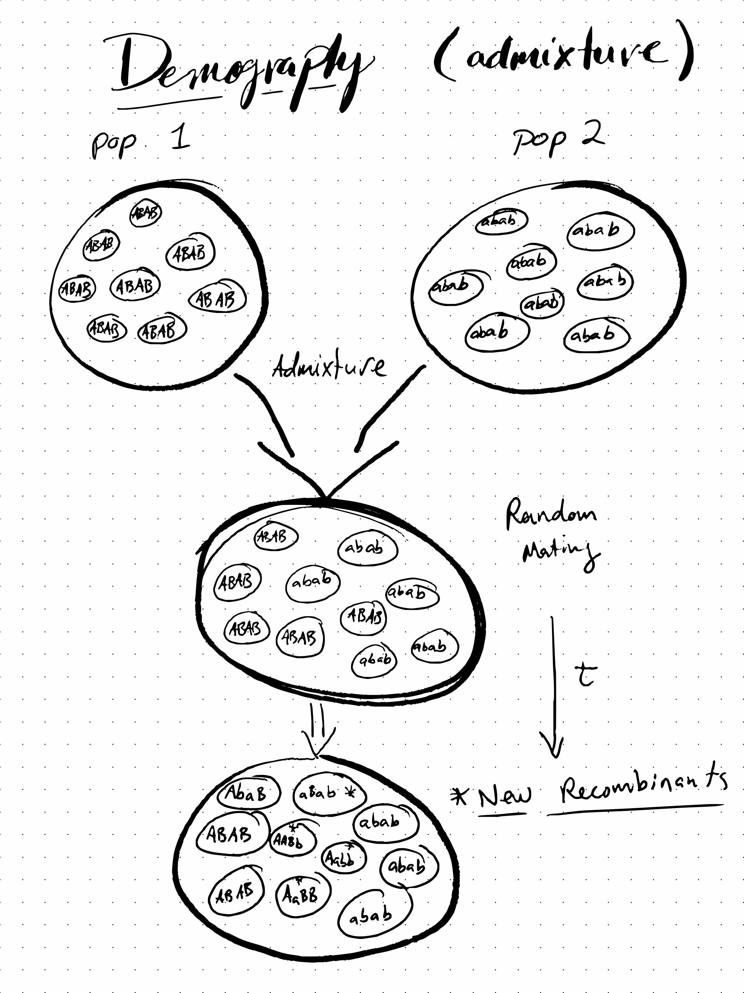
In fact, this is the focus of our Zapf Dingbat LD Exercise that we will go through in class. In brief, we will explore how LD is generated between two loci (\(\mbf{A}\) and \(\mbf{B}\)) by admixture between two populations that are fixed for the alternative alleles at these loci (i.e., where one population has only \(AB\) haplotypes, while the other has only \(ab\) haplotypes; see Figure 1). We will then explore how recombination in the admixed population breaks down LD over time.
Selection at two loci
Lastly, we will explore how selection at two loci can influence LD, and much more. Specifically, we walk through 3 selection scenarios:
- Positive selection (hitchhiking of a neutral allele).
- Overdominance and the “cost of recombination”.
- Epistasis with synergistic alleles, fitness valley crossing.
I currently have a .ppt presentation illustrating these three selection scenarios and their effects on LD that I present in class. I plan to update this webpage with a series of animations and figures to complement the lecture material. Please bear with me as I slowly develop this online notes page.
- Selection at multiple loci can have strong and diverse effects on LD!
- There is much more to selection than what we learned in our simple 1-locus models earlier in the course.
- When two or more loci are involved, we can get a variety of interesting evolutionary dynamics, including hitchhiking, the evolution of reduced population mean fitness, and much more.
So why all the fuss about LD?
It is precisely because LD is affected by diverse evolutionary processes (drift, demography, selection, linkage), that it can serve as an important signal in DNA sequence data.
However, this also makes it difficult to distinguish between the combined effects of these processes acting simultaneously. We cannot immediately attribute causation to one possible factor over another.
LD gives us a tool for studying more common smaller-effect variants, as opposed to pedigree/crossing based approaches to large-effect variants.
LD gives us statistical power!
- If all polymorphisms were independent, association studies would have to investigate each separately.
- LD makes linked variants highly correlated, causes smaller-effect variants to “show up” in genome wide association studies.
Genome-wide patterns of LD
Again, this material is currently presented mostly via .ppt in class. I plan to update this space with new material when I get the chance. Please bear with me.